User: If 1 maps to 7, 9 maps to 63, and 4 maps to 28, then what does 6 map to?
AI’s response: 42.
In-context learning (ICL) is when a model learns at inference-time to do a task from examples given in its prompt. You show it a few input-output pairs, and given a new input, it produces the right output. The model learns what to do on-the-fly all within the forward pass. Traditionally, “learning” is an offline process, where one trains a model on data while updating the weights based on feedback. In ICL, the weights don’t change, but something in the forward pass is doing work that seems to resemble learning.
Large language models exhibit this capability. The question is: how? Studying ICL systematically in large frontier models is very difficult. In order to make progress, I conduct a mechanistic analysis of ICL in the simplified ICL linear regression setting introduced by Garg et al. (2022).
I'll first describe the ICL linear regression setting informally. The goal in this setting is to teach the model to “solve” linear regression based on novel inputs in the prompt. Every time we prompt the model, the model is presented with a fresh dataset of 20 $(x_i,y_i)$ pairs that is hasn't seen before and an $x_q$, with the goal of predicting $y_q$.
The fresh dataset is generated from a random linear function $y=w^Tx$, where $w$ is generated randomly each time.
Because $w$ is generated randomly each time, the model cannot memorize any specific $w$. The intention is that the model must learn a general procedure utilizing the 20 $(x,y)$ pairs to “solve” linear regression, and use that solution to accurately predict $y_q$. It then executes this general learning procedure in its forward pass to accurate solve novel inputs.
Experimental Setup
I adopt the ICL linear regression setup from Garg et al. (2022). This setting has been widely used — Akyürek et al. (2022), von Oswald et al. (2023), Ahn et al. (2023), Raventós et al. (2023), Panwar et al. (2024), Collins et al. (2024), and Hill et al. (2025), among others.
Task. At each training step, I sample a fresh weight vector $w \sim \mathcal{N}(0, I_d / d)$ with $d = 5$, defining a linear function $y = w^\top x$. I then sample $n = 20$ in-context inputs $x_i \sim \mathcal{N}(0, I_d)$ and compute their labels $y_i = w^\top x_i$. A separate query $x_q \sim \mathcal{N}(0, I_d)$ is sampled, and the model is supervised to predict $y_q = w^\top x_q$. The input is a flat sequence of $2n + 1 = 41$ tokens: $[x_1, y_1, x_2, y_2, \ldots, x_{20}, y_{20}, x_q]$. The weight $w$ is hidden from the model at all times. Because $w$ is resampled every step, the model cannot memorize any specific $w$ and must instead learn a general procedure for solving linear regression from the in-context examples. The default setting uses $n/d = 4$; I vary this ratio in later experiments.
Model. Standard decoder-only transformer blocks with pre-norm layernorm, 4 attention heads, hidden dimension $d_\text{model} = 128$, feedforward dimension $d_\text{ff} = 256$, GELU activations, and learned positional embeddings. Each $x_i$ is embedded into the residual stream via a linear projection from $\mathbb{R}^d \to \mathbb{R}^{d_\text{model}}$; each $y_i$ is placed as a scalar in the first coordinate of its token position and embedded through the same input projection. The final $y_q$ prediction is read from a linear projection applied to the residual stream at the $x_q$ position after the final layer. Depth (number of transformer blocks) varies across experiments and is the main variable under study — I train models at depths 1, 2, 3, 4, 5, 6, and 8.
Training. MSE loss on $y_q$. Adam optimizer with learning rate $3 \times 10^{-4}$ and a OneCycleLR schedule (pct_start = 0.1), batch size 256, trained for 200k steps unless otherwise noted. The extended-training analysis in Part 2 runs to 400k–800k steps. The primary seed for all Part 1 analyses is 42; cross-seed replications use seeds 100 and 200. The 3L extended-training analysis additionally uses seeds 500 and 600.
Evaluation. By default, evaluation inputs are drawn from the same $\mathcal{N}(0, I_d)$ distribution as training. The out-of-distribution stress tests sweep alternative covariance structures for the in-context inputs $x_i$: diagonal anisotropic (condition number 100), strongly diagonal (condition number 10,000), and correlated non-diagonal. The weight $w$ is always drawn from the same training prior.
Part 0: The one-layer transformer
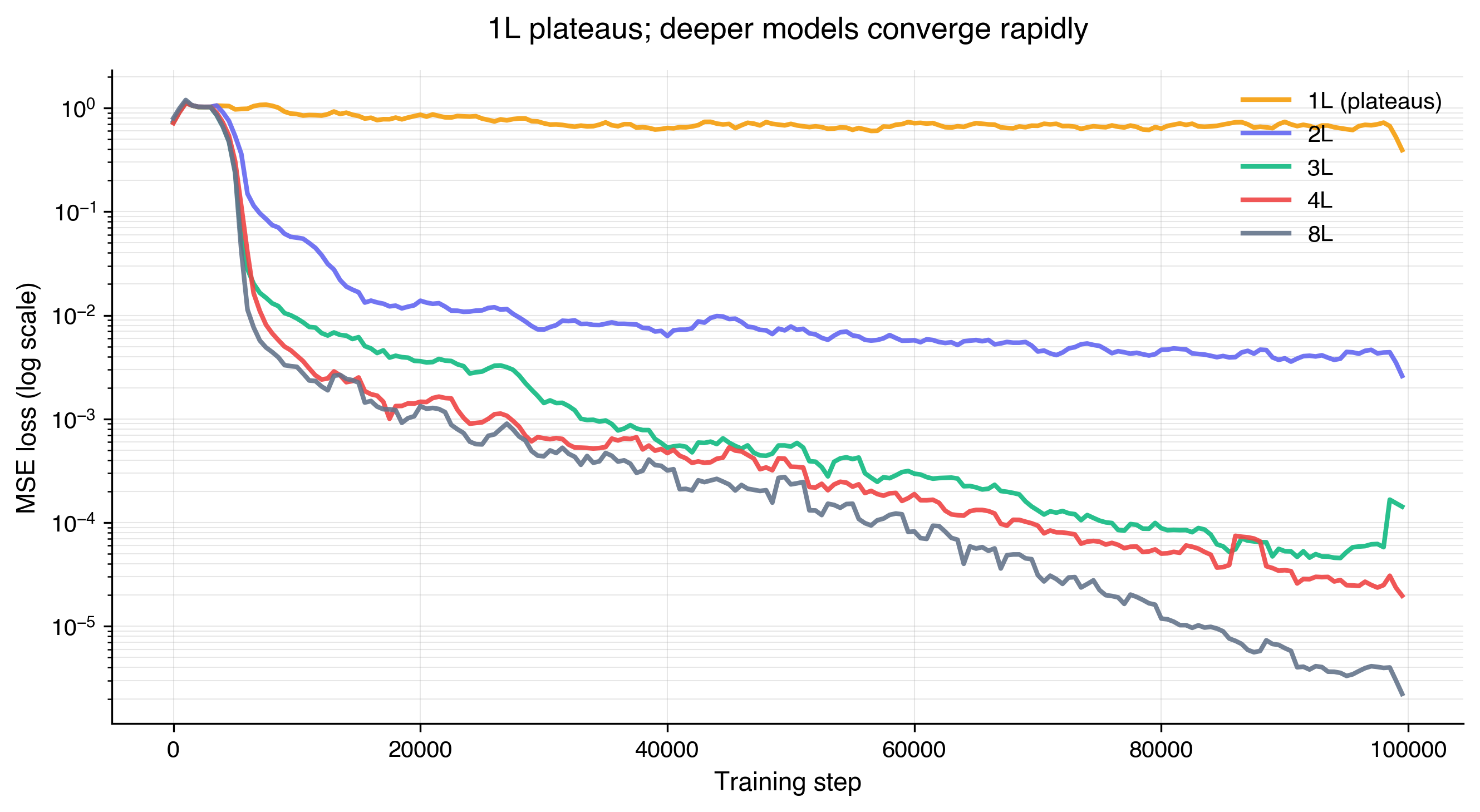
Just to get a baseline, we train models at various depths and plot the MSE loss. As we can see, relative to other models, the 1L transformer plateaus quickly and never improves. We will provide an explanation in later sections about why the 1L model is insufficient for the model to learn linear regression in the ICL setting, but for now we will proceed with an analysis of deeper models.
Part 1: Reverse-engineering the two-layer transformer
The 2L transformer model was the the minimal depth that seemed to learn something non-trival in the ICL linear regression setting. Our goal is to characterize and attempt to pin down precisely what it has learned. Prior works have characterized the 2L transformer in a behavioral sense, with preliminary explanations for what is internally happening algorithmically. In this section, we will carefully reverse-engineer various sub-layers of the 2L transformer to get further algorithmic and mechanistic insight.
Behavioral baseline
Prior work from Akyürek et al. (2022) established that shallow transformer models behave like ridge regression. By "behave", I mean in a black-box sense: given the same inputs, the model's outputs roughly match the ridge regression solution's outputs. It can be shown that 2-layer transformers matched a ridge regressor at a specific $\lambda$, and that the best-match $\lambda$ shifted with added label noise in the way ridge regression predicts. This is a behavioral signature consistent with the model implementing something ridge-like.
The behavioral analysis serves as a valuable baseline. However, just because something behaves like something else, doesn't mean their internals are the same. We will pursue this hypothesis further at an algorithmic level. That is, given that our model seems to behave like ridge regression, can we find sufficient evidence to claim that it is indeed executing ridge regression algorithmically? By "algorithmic" level, we mean that our model is actually executing the same steps as ridge regression would. If we can find sufficient evidence that our model is executing ridge regression's steps algorithmically, we can be more confident in the claim that our model has re-discovered the ridge regression algorithm. This would indeed be interesting, as it would mean that this algorithm is somehow encoded into the weights, and used to accurately make predictions on novel inputs in its forward pass.
Linear probing
To further investigate our hypothesis, we test if any of ridge regression's quantities are "present" within the model's computation. In other words, we introspect the model's sub-layers to see if we can find evidence that it contains representations of ridge regression.
Recall that the closed-form solution for ridge regression is:
$$w = (X^TX + \lambda I)^{-1}X^Ty$$
Some reasonable quantities of ridge regression to look for are $X^TX$, $X^Ty$, and $w$. In order to test if these quantities are "present" at some point internally in the model, we adopt a standard methodology known as linear probing, first proposed by Alain & Bengio (2016).
The intuition behind linear probing is that we test to see if there exists a linear mapping from the per-layer activations to the target quantity. If the probe's prediction aligns strongly with the target quantity, then this means that the quantity is easily accessible to the model in the sense that it is only one linear mapping away from being retrieved.
Here are the results of this linear probing. I denote the two layers of our 2L transformer model as L0 and L1, along with probing results at sub-layer attention and MLP.
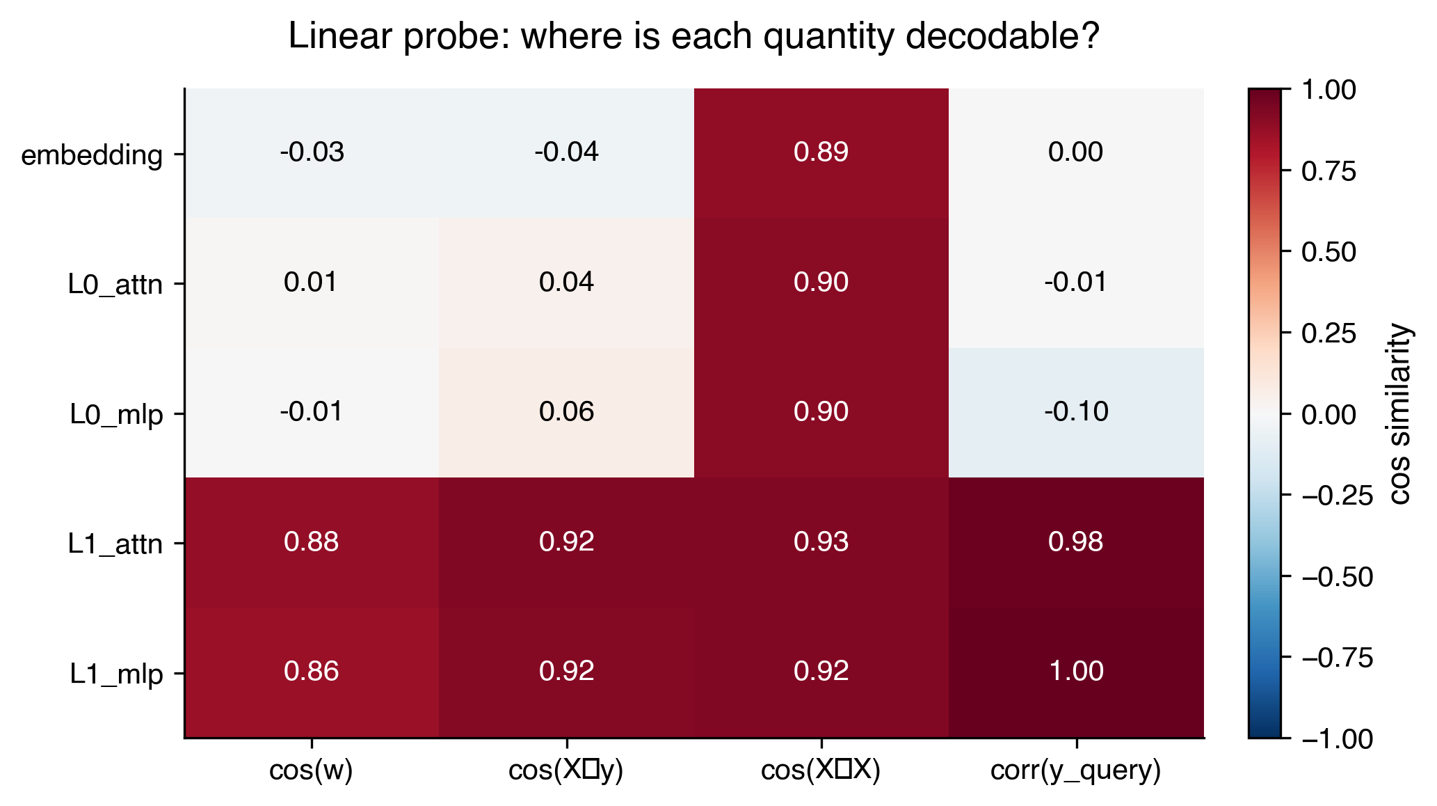
We see that $w$ and $X^Ty$ are readily accessible right after L1’s attention mechanism. What’s intriguing as well is their sharp emergence. They were barely linearly decodable after L0 MLP. This also suggests that L1 attention is doing something pretty useful. We will investigate this more carefully in a later section.
Activation patching
To further strengthen the claim that L1 attention is where a sharp transition occurs, I use a causal technique known as activation patching.
In activation patching, we take the current model (known as the recipient), patch in a different activation output (from a donor) in the residual stream, and we measure the impact on the final prediction.
In this case, both the recipient and donor receive different datasets in their prompt, but the same $x_q$. I perform activation patching at various sub-layers and see how the predictions change.
Results (n=200 donor→recipient pairs):
| Patch location | MSE to donor's answer | MSE to recipient's answer | Interpretation |
|---|---|---|---|
| embedding | 2.34 | 0.0009 | → Recipient |
| L0_attn | 2.25 | 0.075 | → Recipient |
| L0_mlp | 2.25 | 0.075 | → Recipient |
| L1_attn | 0.0009 | 2.35 | → Donor |
| L1_mlp | 0.0009 | 2.35 | → Donor |
We see results matching our linear probing results. A sharp transition occurs at L1 attention. Patching the $x_q$ residual stream before L1 attention has no effect on the final prediction (the model continues to output the recipient's answer). But patching at L1 attention or later flips the prediction entirely to the donor's answer. This tells us that the task-relevant computation is happening at L1 attention: the pre-L1 residual stream doesn't carry enough information to determine the answer, while the post-L1 residual stream fully determines it.
What is L0 doing?
With the understanding that L1 attention is clearly important, let's take a step back and understand the role of L0. L0 is definitely doing something, but it isn't apparent from the linear probing and activation patching experiments. When ablating any single L0 attention head (by ablation, I mean setting the output of the head to 0), the final MSE explodes by 46-801x across various seeds. Each L0 attention head is clearly contributing meaningfully to the final prediction.
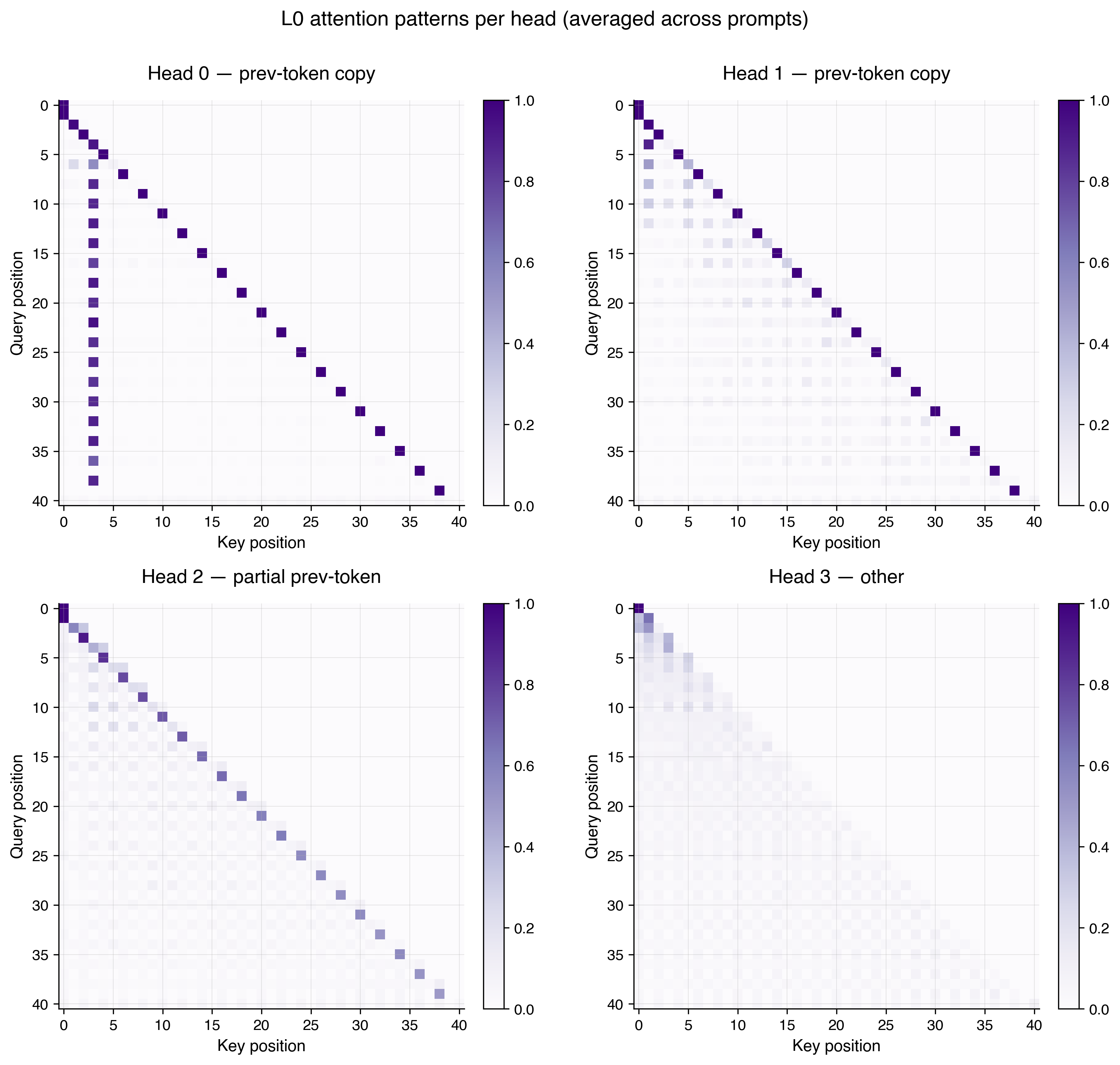
What I found is a pattern similar in nature to what is described in Olsson et al. (2022)'s work on induction heads. Recall that the input prompt is of the form $[x_1, y_1, x_2, y_2, \ldots]$, where $x$-tokens sit at even positions and $y$-tokens at odd positions. Based on the attention patterns and V-projections in L0, I found that two heads are responsible for "mixing" each $x_k$ and $y_k$ pair together. Under the interpretation that attention performs a linear combination of V-projected residual streams, I found that each $y_k$ token attends almost entirely to the preceding $x_k$ token, with the effective V-projection being approximately the identity. The result is that each $x_k$ gets directly copied into the $y_k$ token's residual stream. What's also interesting is that each $(x_k, y_k)$ pair is mixed independently, with no cross-example interaction in L0. L0 is a per-example setup phase for the computation performed in L1 attention.
We know from linear probing that $X^\top y$ is linearly decodable in the L1 attention residual stream. It turns out that L1 attention alone cannot perform this computation without L0's help. To see why, $X^\top y = \sum_k x_k y_k$ requires multiplying each example $x_k$ by its corresponding label $y_k$, then summing across $k$. A single attention layer cannot produce this bilinear combination from separated $x$ and $y$ tokens, because doing so requires first pairing each $x_k$ with its $y_k$ (which L0 does via the copy mechanism above), before aggregating across $k$ (which L1 then does with a near-uniform attention pattern). This is why the 1L transformer from Part 0 failed to learn the task.
Examining L1 attention
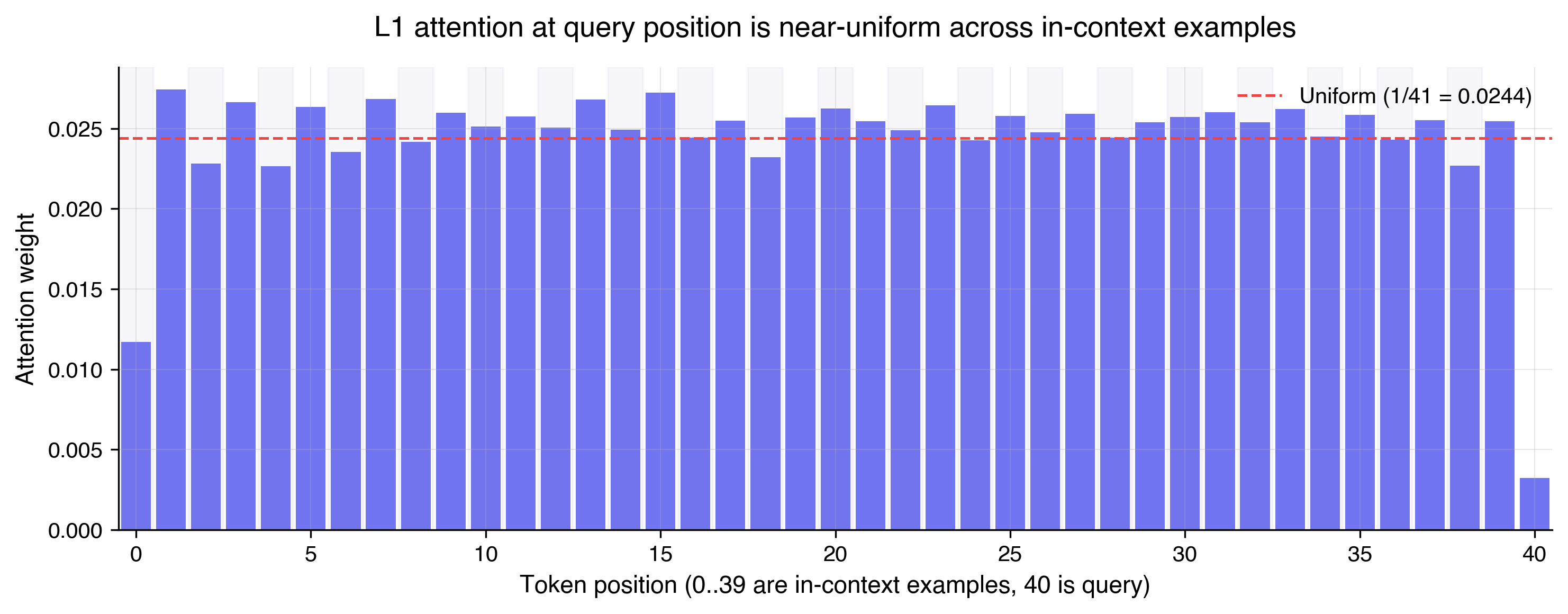
Now that the role of L0 is better understood, we now revisit L1 attention, which is the heart of the model. Reusing our intuition that attention performs a linear combination of V-projected residual streams, we now expect L1 attention to be attending across all of the examples, which are now colocated, thanks to L0. The attention pattern in L1 I found is near-uniform, but not exactly uniform. One way to quantify "near-uniform" is to measure the entropy of the attention distribution. Entropy is maximized when weights are spread equally across all positions, and drops as the distribution concentrates on a few positions. L1 attention's entropy is about 98% of the maximum possible, meaning the weights are spread nearly equally across the 20 examples, but not perfectly so. Interestingly, when I replaced L1 attention with an exactly uniform attention pattern, the final MSE blows up by 1202x. It seems that the near-uniform pattern suggests that L1 attention values all of the examples roughly equally, while some computation is encoded in the slight deviations from uniform.
One interesting hypothesis I had in attempts to characterize L1 attention further is a "streaming computation" hypothesis. The idea here is that because we are using causal attention, perhaps L1 attention is building up the computation of $w$ incrementally across the examples. To test this, I linearly probed for incremental results of $w$, but did not find anything conclusive. It's an open question and future work to more accurately characterize L1 attention.
The role of L1 MLP
As a sanity check, like the previous sub-layers, I confirm that the L1 MLP actually matters in computing the final result. If I take L1_attn's output and apply the model's readout layer directly (skipping L1_mlp), the prediction correlates with $y_\text{true}$ at 0.986. But the MSE is 0.68, compared to the model's final MSE of 0.001. The direction is right; the scale is wrong.
So clearly the L1 MLP is doing something useful with respect to the final prediction. To characterize what it's doing, I fit a series of simple functions to approximate L1_mlp's input-output behavior, and measure how close each approximation gets to the model's actual final MSE.
| Correction | MSE vs $y_\text{true}$ |
|---|---|
| Scalar rescale ($\alpha \approx 0.56$) | 0.038 |
| Affine | 0.037 |
| Quadratic | 0.037 |
| Actual L1_mlp | 0.001 |
A simple scalar rescale gets MSE down from 0.68 to 0.038, capturing most of the correction L1 MLP applies. Adding affine or quadratic terms barely improves on this. But the actual L1 MLP achieves 0.001, nearly two orders of magnitude lower. This tells us that the dominant thing L1 mlp does is apply a scalar rescale, but the remaining gap to the model's final MSE requires a genuine nonlinearity that a low-order polynomial fit doesn't capture.
But beyond $X^\top y$ and $w$, we have yet to find evidence that the model is computing the inverse $(X^\top X + \lambda I)^{-1}$, which is the last significant computation in ridge regression. If we can find it, perhaps we can start to claim that our model has indeed rediscovered ridge regression and is performing it at an algorithmic level.
Despite extensive probing, I was not able to find evidence that the model computes this inverse in the general sense. This was surprising to me because the model seems to be computing partial components of ridge regression, like $X^\top y$, but it seems like the pressure during training forces the model to find a clever shortcut related to the distribution the data is sampled from, and it performs this shortcut at L1 MLP. I investigate this claim further in the next section.
Simplifying the inverse computation
Recall that $X$ are isotropic Gaussian inputs. Since each value is sampled from $\mathcal{N}(0, 1)$, you can expect that $\mathbb{E}[X^\top X] = n I$, where $n$ is the number of examples. This implies that: $$(X^\top X + \lambda I)^{-1} \approx (nI + \lambda I)^{-1} = \frac{1}{n + \lambda} I$$
Multiplying $X^\top y$ by this scalar value $\frac{1}{n + \lambda}$ is approximately the ridge solution, which is exactly the role of L1 MLP. Through this derivation, we have shown that the matrix inversion degenerates to scalar multiplication under the isotropic Gaussian data distribution.
A natural hypothesis now is that the model hasn't actually learned the final inverse computation, but instead found a shortcut rather than fully rediscovering ridge regression. We will pursue this hypothesis momentarily. The outcome that the model found a training distribution shortcut isn't all that surprising, but what is interesting is that the model appeared to at least partially compute ridge regression. A natural instinct is to try to train on more data (beyond just the isotropic Gaussian distribution), which is definitely worth doing, but I didn't do it for this blog. What I hypothesize is that the updated model would find new shortcuts of the distribution to exploit, and so we'd in some sense be moving goalposts. So instead, we opt to study the isotropic Gaussian distribution, which matches the experimental setup of prior work.
The model is a mimic, not a ridge regressor
We now confirm our suspicions above about our model finding a training distribution-specific shortcut in L1 MLP.
First, I confirm that when doing inference with datasets generated from anisotropic distributions, the model MSE explodes, while a real ridge regression still solves the problem successfully. We see that the scalar trick that the model learned cannot compensate for a real $X^\top X$ inverse. The eigenvalue structure of $X^\top X$ for anisotropic distributions is too different from the isotropic case that the model was trained on.
| Covariance | Condition # | Model MSE | Ridge MSE | Ratio |
|---|---|---|---|---|
| Identity | 1 | 0.0009 | 0.000001 | ~1000× |
| Diagonal anisotropic | 100 | 0.37 | 0.000003 | ~10⁵× |
| Strongly anisotropic | 10,000 | 30.7 | 0.00003 | ~10⁶× |
| Correlated | ~21 | 0.064 | 0.000001 | ~10⁵× |
Second, to further characterize the dependence on training distribution, I train a model from scratch where $x$ is sampled solely from a Rademacher distribution (each coordinate of $x$ is $+1$ or $-1$ with equal probability). This distribution still has the same $\mathbb{E}[X^\top X] = nI$ as Gaussian, but it is discrete rather than continuous. This is to test whether the model's mechanism depends on the inputs being continuous, and also to check whether the model might just memorize solutions. For our $d=5$, it's plausible that the model could memorize the $2^5 = 32$ possible $y$-outputs for each distinct $x$-input pattern, since the space of $x$-inputs is small.
What we find is that models trained on these different training distributions all successfully learn (as shown by low MSE on the training distribution). What is different is that for the Rademacher model, we lose the linear decodability of $w$. I hypothesize that the Rademacher-trained model is no longer attempting to represent something resembling $w$, but has instead found a shortcut more indicative of memorizing solutions. Not shown in this table, but when I evaluate a Rademacher-trained model on Gaussian inputs, the MSE explodes to 0.25 (~416×). This implies there is no real linear interpolation learned in the Rademacher-trained model. In fact, the training process has no motivation to learn this concept, since the discrete distribution rewards memorization just as well.
| $x$ distribution | cos($w$, L1_mlp) | MSE (training distribution) |
|---|---|---|
| Gaussian (original) | 0.88 | 0.001 |
| Uniform | 0.88 | 0.0003 |
| Laplace | 0.90 | 0.0009 |
| Rademacher (seed 42) | 0.53 | 0.0006 |
| Rademacher (seed 100) | 0.14 | 0.0013 |
| Rademacher (seed 200) | 0.69 | 0.0004 |
Taken together, these results show that our 2L model has not re-discovered ridge regression. It has found a shortcut that exploits the isotropy of the training distribution to collapse the matrix inverse into a simple scalar multiplication. This shortcut reproduces ridge's outputs on isotropic inputs, but breaks catastrophically the moment the input distribution changes. The model behaves like ridge, but it does not implement ridge on an algorithmic level.
What's interesting is that the model does develop partial representations of ridge. We found $X^\top y$ and $w$ as linearly decodable quantities in the residual stream, which are genuine components of ridge's computation. The model isn't doing something unrelated to ridge and getting lucky. It's doing part of ridge and then taking a distribution-specific shortcut for the part that's hard. We were able to pinpoint precisely where this substitution happens: at L1 MLP. The broader takeaway isn't just that the model fails OOD, but that behavioral matching to a classical algorithm can hide this kind of partial-implementation-plus-shortcut structure, which is only visible through mechanistic analysis.
Part 2: Scaling depth beyond the two-layer transformer
We now investigate what happens when we scale beyond two layers. The basic quantitative motivation is straightforward: we saw in an earlier figure that MSE drops by orders of magnitude with depth (from approximately $10^{-2}$ at 2L to $10^{-5}$ at 8L, at 100k steps). It will also be interesting to see what findings and intuitions from the 2L transformer experiments generalize, and which need to be re-worked. Note that this section is preliminary, but I report some initial findings that I found surprising.
Two natural intuitions frame what we might expect. From a computational perspective, more layers give the model room to perform the iterative inverse of $(X^\top X + \lambda I)$ directly, rather than taking the 2L shortcut. From a scaling laws perspective, scaling tends to improve model properties beyond just the training loss, including out-of-distribution behavior.
What I found contradicts both perspectives in an interesting way. The algorithm that the model discovers changes qualitatively between 3L and 4L, but the distributional failure mode from Part 1 persists through this internal mechanism change. Increasing depth changed how the model produced its predictions, but without changing which distributions its predictions are accurate on.
The primal to dual phase transition hypothesis
Figure
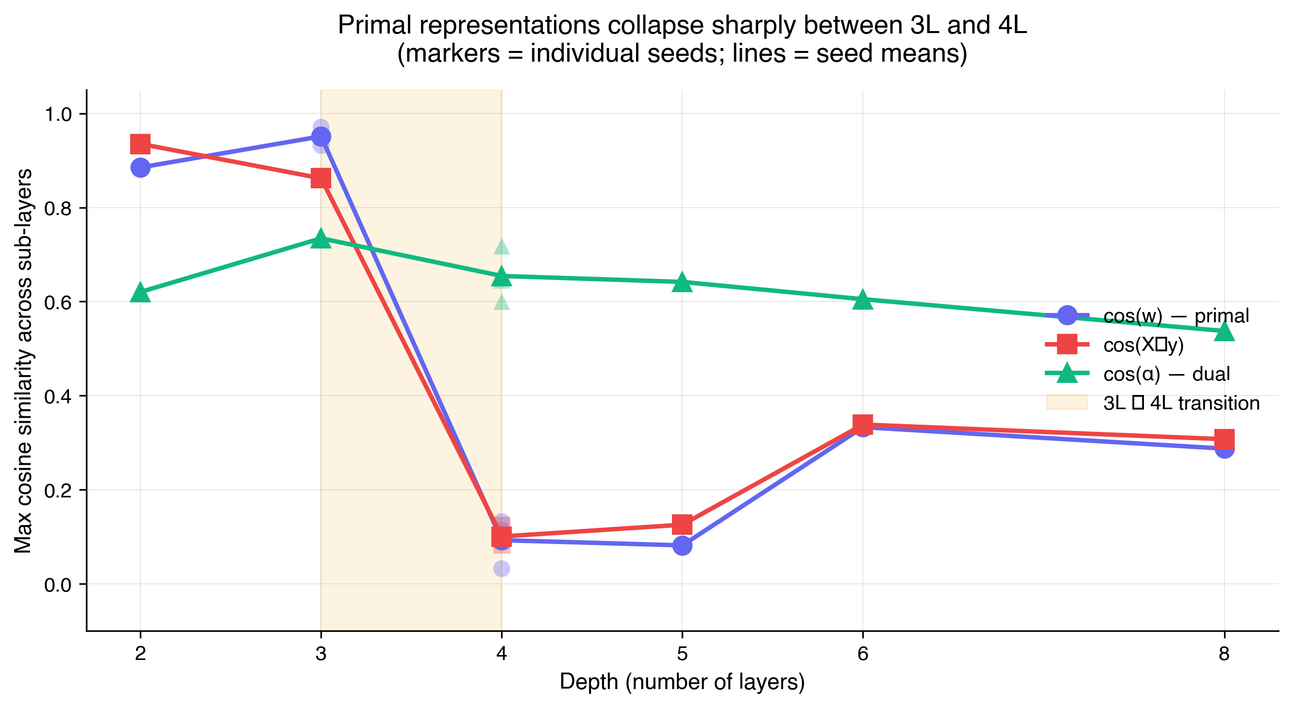
| Depth | cos(w) | cos(X⊤y) | cos(α) |
|---|---|---|---|
| 2L | 0.89 | 0.94 | 0.62 |
| 3L | 0.93, 0.97 | 0.86, 0.86 | 0.73, 0.74 |
| 4L | 0.11, 0.03, 0.13 | 0.12, 0.10, 0.08 | 0.60, 0.72, 0.65 |
| 5L | 0.08 | 0.13 | 0.64 |
| 6L | 0.33 | 0.34 | 0.61 |
| 8L | 0.29 | 0.31 | 0.54 |
2L, 5L, 6L, 8L: single seed (42). 3L: two seeds to confirm primal regime. 4L: three seeds to confirm the collapse replicates.
[X1] When we scale the depth of the model from 2L to 4L and beyond, the linear decodability of w and X⊤y collapses — strong evidence that the model has abandoned the primal formulation of linear regression. What's striking is that this transition is sharp: it happens between 3L and 4L, not gradually. A preliminary hypothesis is that the model has transitioned from the primal formulation to something dual-shaped. [/X1]
[X2] The implication of this is interesting. It suggests that the model's internal representations no longer treat w — the hidden weight vector that actually generated the data — as the computational object of interest. This is counter-intuitive: w is a single compressed summary of everything needed to reproduce the line underlying the data. But given more depth, the model sharply moves away from representing it. On the surface, depth adds capacity; more fundamentally, it gives the network access to algorithmic forms that shallower networks cannot reach. [/X2]
[X3] Let's briefly review the dual formulation. The prediction is expressed directly as a weighted combination of training labels: ŷ = Σᵢ αᵢ(x_q) · yᵢ. The per-example weights αᵢ depend on the query and are derived from a kernel function K(xᵢ, x_q) that measures similarity between each training input and the query. For linear regression with a linear kernel, the primal and dual forms give identical predictions — but they're different computations. Primal builds w once and applies it; dual never explicitly represents w, and instead weights each training label by how similar its x-value is to the query.
Why the dual form matters conceptually: the kernel K can be any similarity function, not just the linear one. Kernel methods generalize linear regression to nonlinear settings precisely by swapping in richer kernels. The dual form is more general than primal — primal is a special case where the kernel happens to be linear. So a model that moves from primal to dual-shaped computation is moving toward the more general form. [/X3]
[X4] To test whether the 4L model is actually doing dual, I probed for α — the per-example coefficient vector that a dual form would compute. Specifically, I computed the α that would correspond to an RBF kernel evaluation between each training xᵢ and the query x_q, and checked whether this vector is linearly decodable from the residual stream. RBF (radial basis function, k(xᵢ, x_q) = exp(-‖xᵢ - x_q‖² / 2σ²)) is the natural guess because softmax attention implements something kernel-like by construction: attention weights are exp(q · k / √d), which under normalized inputs is closely related to an RBF kernel.
The result is suggestive but not conclusive. cos(α) rises from 0.62 at 2L to 0.60-0.72 across 4L seeds — higher than the 2L baseline but not dramatically so, and the probe is a crude one (α depends on x_q, so decoding a single α vector from the residual stream is a rough approximation). What's currently resolved in the literature: Collins et al. 2024 proved that single-layer softmax attention trained on linear regression ICL implements kernel regression with a specific bandwidth. What remains unresolved: whether trained multi-layer transformers implement kernel regression with characterizable bandwidth, and what the precise kernel form is at each depth. This blog contributes an empirical observation — that a sharp transition to a non-primal regime occurs at a specific depth — without resolving the kernel characterization question. [/X4]
The inductive bias of attention
[X5] As we noted earlier, the attention mechanism computes, at each query position, a weighted sum of value-projections of other tokens. Its native computational shape is output = Σᵢ softmax(q · kᵢ) · vᵢ — structurally identical to the dual form ŷ = Σᵢ αᵢ(x_q) · yᵢ. Dual regression is what attention natively computes. Primal regression, by contrast, requires the model to synthesize a weight vector w as an explicit object in the residual stream and then apply it to the query through later layers — a shape that doesn't naturally emerge from weighted-sum operations. Primal fights the architecture; dual flows with it.
With only two attention layers, dual is architecturally inaccessible: implementing it cleanly would require one attention operation to compute per-example coefficients and another to aggregate labels weighted by those coefficients — and 2L's first layer is already occupied with more basic aggregation work (building representations like X⊤y that subsequent layers operate on). Four layers relaxes this constraint. Dual becomes implementable, and the optimizer appears to prefer it. [/X5]
[X6] Recent literature partially converges on this picture. Collins et al. (2024) prove that single-layer softmax attention trained on ICL regression implements kernel regression with a specific bandwidth. Akyürek et al. (2022) show behaviorally that depth correlates with different classical-algorithm matches (shallow → ridge, deeper → OLS). von Oswald et al. (2023) hand-construct transformers that implement gradient descent on linear regression. He et al. (2025) analyze softmax kernel regression in extended settings. What's converging: single-layer characterizations and behavioral depth-effects. What remains open: what trained multi-layer transformers mechanistically implement, and whether the primal-to-dual-like transition observed here is a general phenomenon. [/X6]
[X7] If this pattern generalizes, it suggests something interesting: when scaling transformer depth on algorithmic tasks, we might expect the optimizer to migrate from computationally-awkward primal-like solutions to attention-native dual-like solutions as soon as depth allows. Depth isn't just adding capacity; it's unlocking access to algorithmic forms that shallower networks can't cleanly implement. Whether this holds for other algorithmic tasks beyond regression is an open problem worth further investigation. [/X7]
Depth vs Capacity
Figure
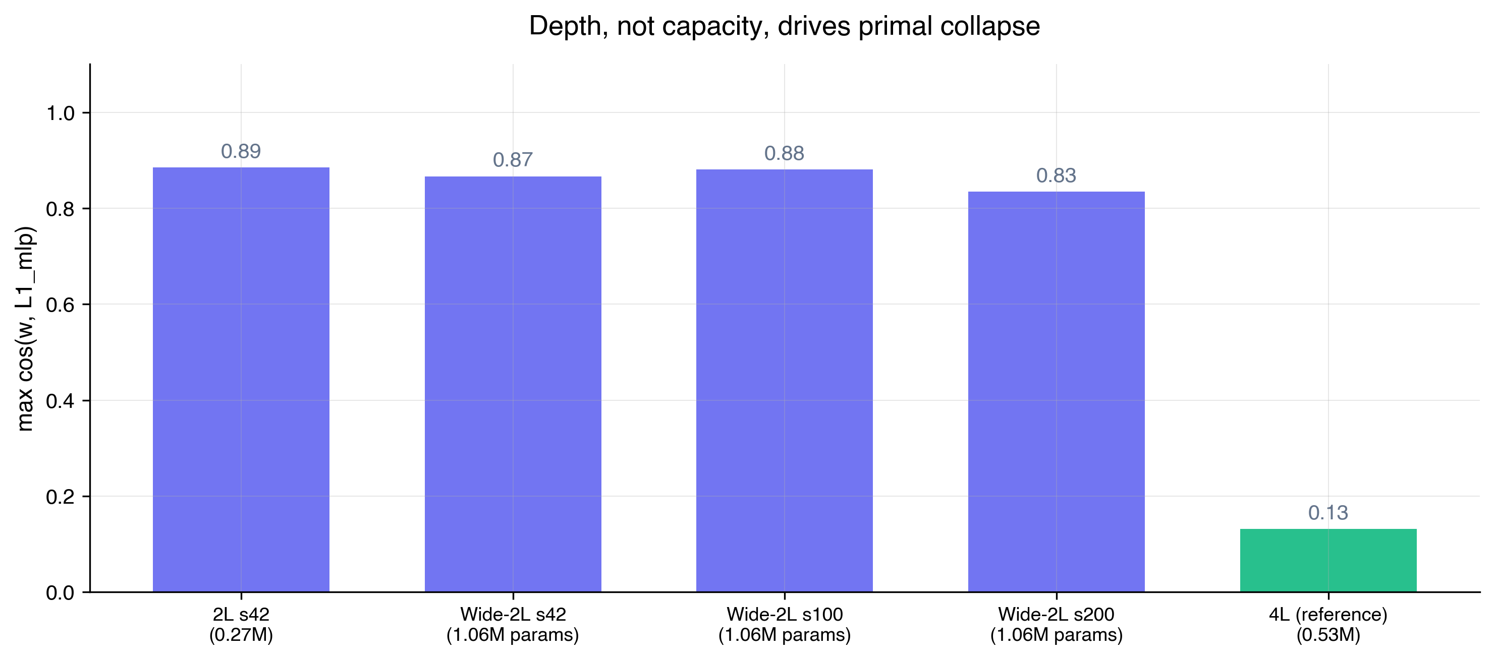
[X8] The most natural objection is that depth isn't really what drives the algorithmic phase change — model capacity is. To test this, I trained three additional 2L models with hidden dimension widened to bring total parameter count to ~1.06M — roughly 4× the standard 2L (0.27M) and 2× the 4L (0.53M). Training setup was otherwise identical: same data distribution, same optimizer settings, same number of steps.
All three wide-2L seeds retained primal structure, with cos(w) in the range 0.83-0.88 — comparable to the standard 2L (0.89) and far above any 4L seed (0.03-0.13). Capacity alone does not drive the transition. It's specifically the addition of attention layers that unlocks the non-primal regime. [/X8]
X⊤y as a strong primal vs dual probe
Figure
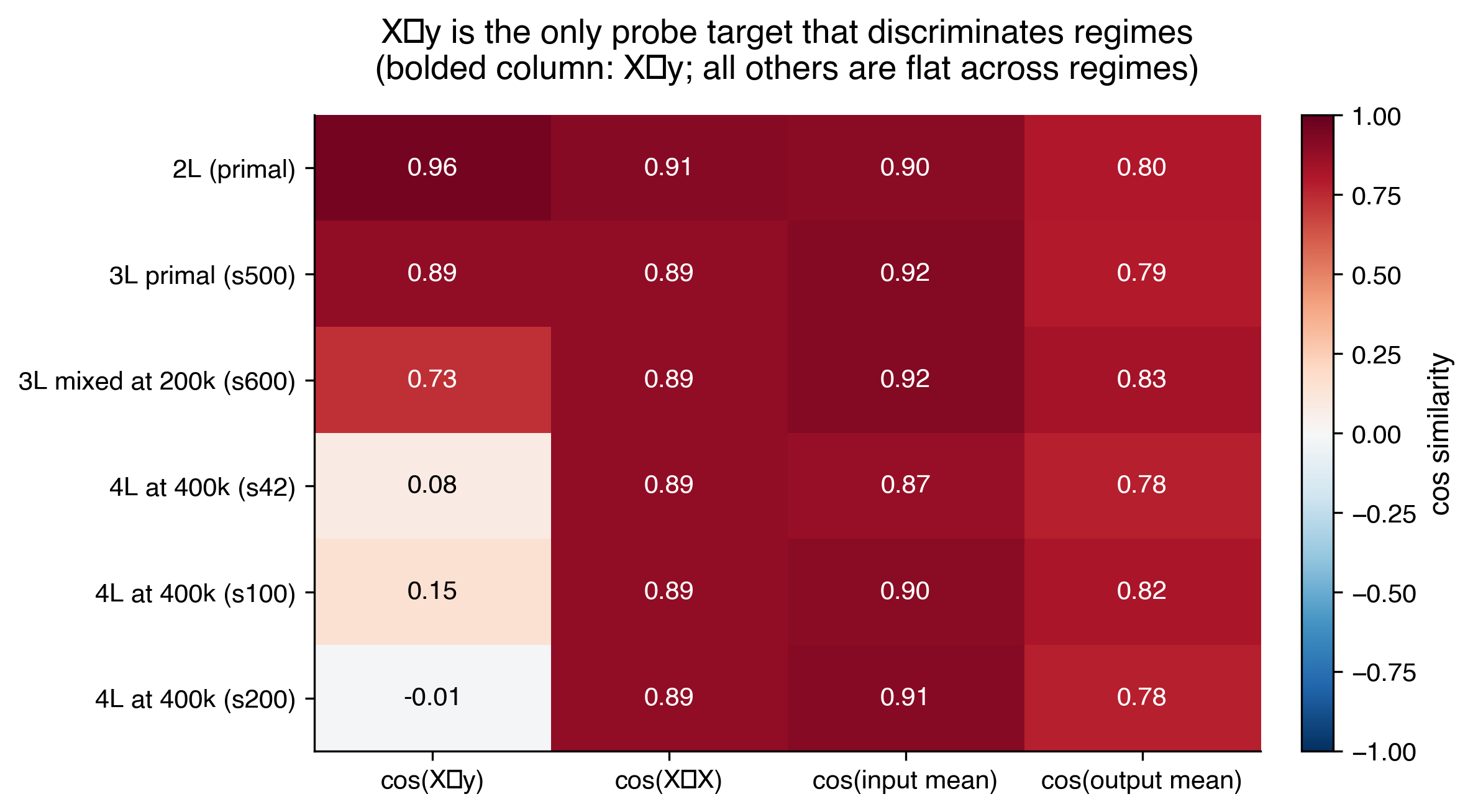
[X9] I haven't seen X⊤y used as a primal/dual diagnostic elsewhere in the ICL mech interp literature, and I think it's worth highlighting for others working in this area. The logic is simple: X⊤y is a genuinely computed bilinear quantity that cannot be recovered from the input embedding alone (unlike X⊤X or first moments, which are nearly distribution-constant under the isotropic prior). Its presence or absence in the residual stream is therefore a meaningful computational signal, not a probe artifact.
The steep drop in cos(X⊤y) between 3L (0.86) and 4L (0.08-0.12) mirrors the drop in cos(w), giving two independent lines of evidence that the primal representation has vanished. While this isn't evidence that the model is definitively computing dual, it is strong confirmation that the model is no longer computing primal. [/X9]
Extended training resolves 3L
Figure
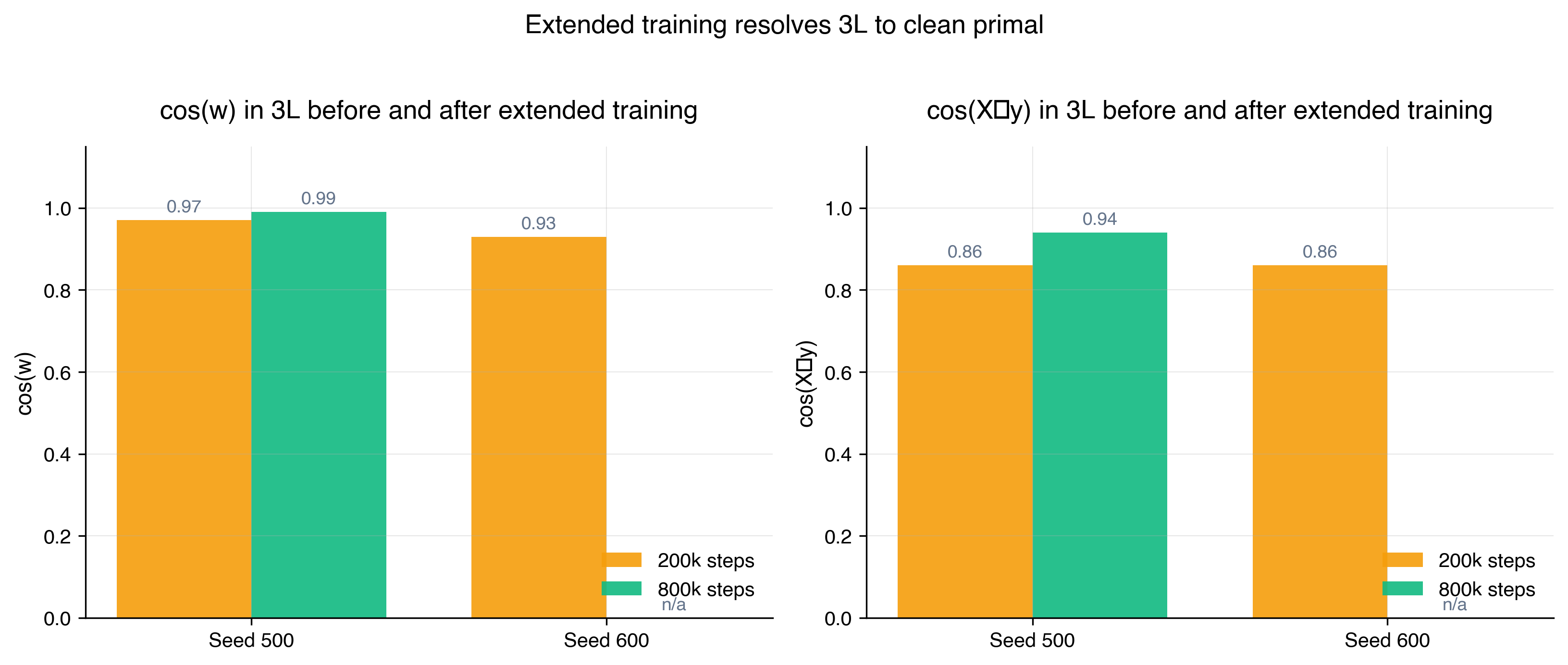
[X10] [FIGURE NEEDED: trajectory plot of cos(w) and cos(X⊤y) over training steps for anomalous 3L seed, showing resolution from ~0.04 to ~0.99 by 800k steps] [/X10]
[X11] My initial analysis of the phase transition between 2L, 3L, and 4L was messy and inconclusive at first. I was training to 200k steps, which is standard across recent ICL papers. At this budget, some 3L seeds looked partial or mixed — one seed showed cos(w) ≈ 0.04, closer to 4L than 3L. This initially suggested 3L might be an unstable transition regime where multiple attractors coexist.
When I extended training to 400k and 800k steps, the anomalous 3L seeds resolved to clean primal (cos(w) = 0.99, cos(X⊤y) = 0.94). The 200k state was transient, not equilibrium. This means the 3-to-4 boundary is deterministic and sharp: 3L converges to primal, 4L converges to non-primal, with no ambiguous regime in between.
On a methodological level, this suggests that mech interp conclusions drawn at standard training budgets can sometimes reflect transitional states rather than what the model has actually converged to. Worth checking on other analyses, particularly near apparent regime boundaries. [/X11]
4L still contains a distributional shortcut
Figure
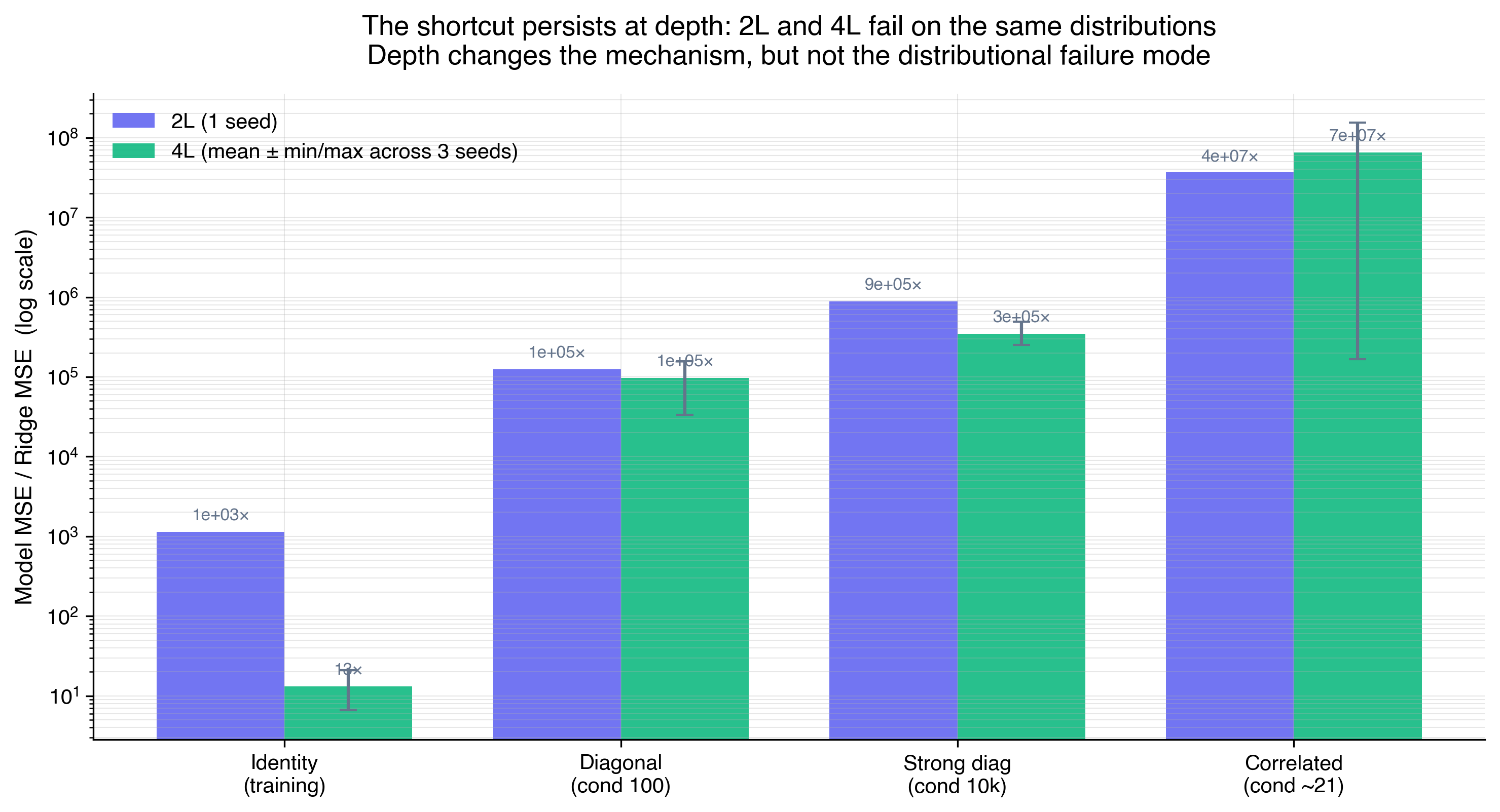
| Covariance | 2L ratio | 4L ratio (mean, range) |
|---|---|---|
| Identity | 1.1e3× | 1.3e1× (6.6–20.9) |
| Diagonal | 1.3e5× | 9.7e4× (3.4e4–1.6e5) |
| Strong diag | 8.9e5× | 3.5e5× (2.5e5–4.9e5) |
| Correlated | 3.7e7× | 6.9e7× (1.7e5–1.5e8) |
[X12] The 4L model finds a different mechanism, but the same failure. I ran the same OOD stress tests from Part 1 on the 4L model across three seeds. On diagonal anisotropic covariance, 4L fails by a factor of 3.4×10⁴ to 1.6×10⁵ relative to ridge regression — the same order of magnitude as 2L (1.3×10⁵). On strongly anisotropic covariance, 4L fails by 2.5-4.9×10⁵, also in the same order of magnitude as 2L (8.9×10⁵). On correlated covariance the comparison is noisier, with high cross-seed variance, but the failure is severe at both depths.
What this means carefully: depth does help on the training distribution — 4L achieves much lower absolute MSE than 2L on isotropic inputs, and its ratio to ridge on that distribution is two orders of magnitude smaller (13× vs 1100×). So depth is genuinely improving in-distribution behavior. What it doesn't do is fix the OOD failure mode: the distributional blind spots carry over through the mechanism change.
This contradicts the scaling-laws folk view that scale fixes generalization. It's a single data point in a toy setting, not a claim about frontier LLMs — but it's a clean existence-proof that a qualitative mechanistic shift can occur without corresponding improvement in distributional robustness. The shortcut persists not because the model failed to change how it computes, but because changing how it computes didn't touch what it's sensitive to. [/X12]
Future work
[X13] Several things in this analysis are unresolved. First, the 4L mechanism itself: I've shown what 4L isn't doing (primal) but not what it is doing at the circuit level. Fully reverse-engineering 4L — identifying which heads compute per-example coefficients, which aggregate, whether there's an induction-head-like structure for kernel regression — is the obvious next step. Second, characterizing the kernel: my α probe is crude, and direct prediction-level comparisons to Nadaraya-Watson regressors at varying bandwidths would likely resolve more than probe-based approaches. Collins et al. 2024 and He et al. 2025 provide theoretical predictions that could be directly tested. Third, scaling up: 8L shows mixed behavior (cos(w) rises to 0.45 across sublayers, suggesting partial primal re-emergence), and the regime beyond 4L is unclear. Whether the primal/dual dichotomy holds at GPT-scale is the biggest open question, and the one where this toy-setting result is most obviously limited. [/X13]
Conclusion
[X14] The headline finding of Part 2: between 3L and 4L, the mechanism by which the transformer solves in-context linear regression changes qualitatively — the explicit weight representation vanishes, and something consistent with dual/kernel-form computation emerges. But the distributional failure mode from Part 1 survives the mechanism change. Depth changes how the model computes, without changing what it's accurate on.
Combined with Part 1, this gives a two-sided observation about ICL mech interp on this toy task. Part 1 showed that behavior matching ridge regression can hide a mechanistically shallow shortcut. Part 2 shows that a mechanistic change can occur without touching the behavioral signature of that shortcut. Neither behavioral match nor mechanism change is sufficient to predict what the model does out of distribution.
For interpretability practice, the lesson is modest but concrete: "the model has learned X" can mean different things in different settings, and interp methodologies that rely on either behavior-matching alone or circuit-finding alone are missing information. Predicting OOD behavior — which is what we actually care about for safety-adjacent reasons — requires both lenses together.
I don't claim any of this generalizes to frontier LLMs. It's one clean observation in a toy setting where everything is visible. But it's a setting where the dissociation between mechanism and distributional behavior is provable, and the existence of the dissociation is, I think, worth carrying forward into how we think about interp at larger scales. [/X14]